Perceptron Class Source Code: https://github.com/kate-kenny/kate-kenny.github.io/blob/main/posts/blog1/perceptron.py
To implement the perceptron algorithm, I used the above source code to create a perceptron class and perform perceptron updates. The specific update is performed using the fit() method of the class. I implimented the update based on the perceptron equation which is as follows:
The fit() method takes two arguments, a matrix \(X\) of features and a vector \(y\) of labels. The method then generates a random weight vector, reffered to as \(w\) in my source code, and then iterates through the possible maximum number of steps to perform the perceptron update. The actual update occurs in the following way. As enumerated in the description of the algoritm, once we have a random set of weights \(w\) we generate a random integer \(i\). From there, we index the feature matrix \(X\) and the label vector \(y\) using that integer \(i\) and perform the update which is, in plain language, as follows. The weights in \(w\) will be updated if the dot product of the current weights and \(x_i\) multiplied by the actual label of the point, \(y_i\) is less than zero. In other words, the weights will be changed if the given weights do not corrently label the point \(x_i\). If that is the case, we add
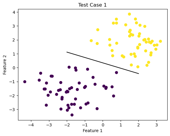
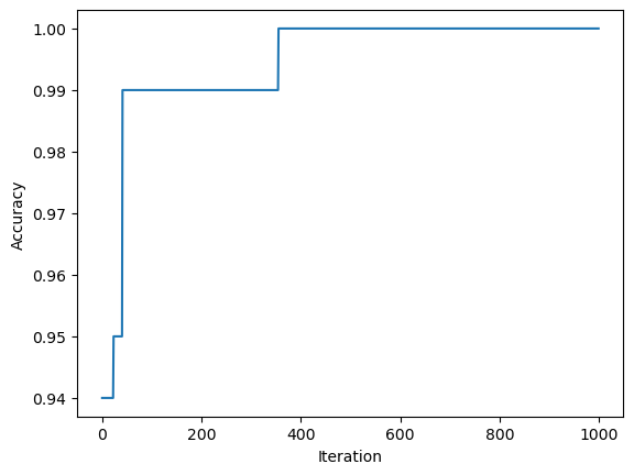
Experiment 1
For the first test case, we are going to run the model on a linearly seperable data set and display the line calculated by the perceptron algorithm to seperate the data points. To do this, I will use the source code provided in class to generate data and then create an instance of my own perceptron class. Finally, we will display the data and seperating line, along with a visual representation of the accuracy over time.
import numpy as npimport pandas as pdimport seaborn as snsfrom matplotlib import pyplot as pltfrom matplotlib import pyplot as plt2%load_ext autoreload%autoreload 2from sklearn.datasets import make_blobsnp.random.seed()n =100p_features =3#initialize X, y, a martix of features and vector of labels respectivelyX, y = make_blobs(n_samples =100, n_features = p_features -1, centers = [(-1.7, -1.7), (1.7, 1.7)])plt.figure(1)fig = plt.scatter(X[:,0], X[:,1], c = y)xlab = plt.xlabel("Feature 1")ylab = plt.ylabel("Feature 2")title = plt.title("Test Case 1")from perceptron import Perceptron#create instance of perceptron class and use the fit() method on X, y initialized above for the first test casep = Perceptron()p.fit(X,y)#draw line from weights found using perceptron algorithmdef draw_line(w, x_min, x_max): x = np.linspace(x_min, x_max, 101) y =-(w[0]*x + w[2])/w[1] plt.plot(x, y, color ="black")fig = plt.scatter(X[:,0], X[:,1], c = y)fig = draw_line(p.w, -2, 2)xlab = plt.xlabel("Feature 1")ylab = plt.ylabel("Feature 2")plt.figure(2)fig2 = plt.plot(p.history)xlab = plt.xlabel("Iteration")ylab = plt.ylabel("Accuracy")
The autoreload extension is already loaded. To reload it, use:
  %reload_ext autoreload
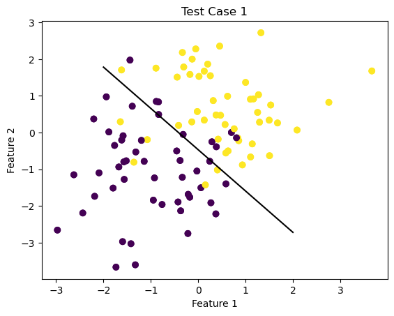
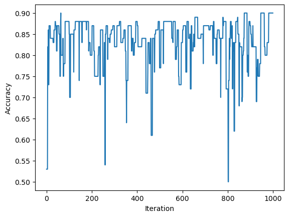
Experiment 2
Now, I am going to explore attempting to use the perceptron algorithm on a non-linearly seperable data set.
First, using a similar process as above, I will generate a data set of non-linearly seperated data and then create another instance of the perceptron class. Then, I will use the fit() method to attempt to generate weights, \(w\), that will produce a line that will try and categorize the data.
Obviously, the algorithm will not converge but I will display the line generated to seperate the data after the full number of max steps has been concluded and also have a visualization of the accuracy throughout this process.
import numpy as npimport pandas as pdimport seaborn as snsfrom matplotlib import pyplot as pltfrom matplotlib import pyplot as plt2%load_ext autoreload%autoreload 2from sklearn.datasets import make_blobsnp.random.seed()n =100p_features =3#initialize X, y, a martix of features and vector of labels respectivelyX, y = make_blobs(n_samples =100, n_features = p_features -1, centers = [(-1, -1), (.5,.5)])plt.figure(1)fig = plt.scatter(X[:,0], X[:,1], c = y)xlab = plt.xlabel("Feature 1")ylab = plt.ylabel("Feature 2")title = plt.title("Test Case 1")from perceptron import Perceptron#create instance of perceptron class and use the fit() method on X, y initialized above for the first test casep = Perceptron()p.fit(X,y)#draw line from weights found using perceptron algorithmdef draw_line(w, x_min, x_max): x = np.linspace(x_min, x_max, 101) y =-(w[0]*x + w[2])/w[1] plt.plot(x, y, color ="black")fig = plt.scatter(X[:,0], X[:,1], c = y)fig = draw_line(p.w, -2, 2)xlab = plt.xlabel("Feature 1")ylab = plt.ylabel("Feature 2")plt.figure(2)fig2 = plt.plot(p.history)xlab = plt.xlabel("Iteration")ylab = plt.ylabel("Accuracy")
The autoreload extension is already loaded. To reload it, use:
  %reload_ext autoreload
Conclusion and Question
Finally, I want to consider the question posed on the assignment page. What is the runtime complexity of a single iteration of the perceptron algorithm update as described by the update equation?
The runtime of the equation is \(O(1)*p\) where \(n\) is the number of data points and \(p\) is the number of features. It doesn’t seem like the number of data points \(n\) would influence the runtime since a single update is only dealing with one randomly selected data point. So, for the update we need to assign the randomly selected points and corresponding weights. Then, for each update, we also take the dot product of each feature with it’s corresponding weight, which is \(p\) operations. Hence, we must multiply the runtime by \(p\).